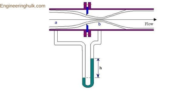
Orifice Meter: Construction, Working, Formula & Uses

An orifice meter measures the flow rate in a full pipe by forcing the fluid through a thin plate with a sharp-edged hole and reading the pressure drop this creates. The fluid speeds up through the hole, so its pressure falls, and the flow rate is proportional to the square root of that pressure difference. It is the cheapest and most widely used of all differential-pressure flow meters, with a discharge coefficient of roughly 0.6 to 0.65 against about 0.95 to 0.99 for a venturi meter. The trade-off is a large permanent pressure loss, which is the pumping energy you pay for the simplicity.

Where the orifice meter sits among flow meters

Flow meters split into several families: differential-pressure meters, variable-area meters such as the rotameter, velocity meters such as turbine and electromagnetic types, and mass meters such as Coriolis. The orifice meter belongs to the first group, alongside the venturi meter and the flow nozzle. All three work on the same physics, an engineered restriction that converts pressure head into velocity head, and all three are covered by the ISO 5167 series. Orifice plates specifically are covered by ISO 5167-2, currently ISO 5167-2:2022, which is the standard a designer actually opens when sizing a plate.

Construction of an orifice meter

An orifice meter is a short list of parts, which is exactly why it is popular.

Part	Function	Typical detail
Orifice plate	Creates the restriction	A flat metal disc, usually stainless steel, with a machined hole. Plate thickness is kept small relative to pipe bore, and the upstream edge must be square and sharp.
Pipe flanges and gasket	Hold and centre the plate	The plate is clamped between two flanges, or carried in a special orifice flange or an orifice fitting that allows plate changes without opening the line.
Pressure tappings	Pick up upstream and downstream pressure	Two small holes drilled through the pipe wall, positioned by one of the three standard schemes described below.
Differential manometer or DP transmitter	Measures the pressure difference	A U-tube mercury manometer in the teaching lab; in industry a capacitance or piezoresistive DP transmitter with a 4-20 mA or digital output.
Impulse lines and manifold	Connect tappings to the instrument	Small-bore tubing with isolation and equalising valves, so the transmitter can be zeroed without stopping the flow.

Why the plate is bevelled on the downstream face

The orifice plate has to do two contradictory jobs. It must be stiff enough not to buckle under the pressure difference, which wants a thick plate, and its bore must behave as a thin sharp-edged opening, which wants a thin one. The answer is a plate of usable thickness whose bore is machined square and sharp only at the upstream face, with the downstream side chamfered at about 45 degrees so the actual cylindrical throat length is short. The bevel always faces downstream. If a plate is fitted the wrong way round, the flow meets a rounded or chamfered entry instead of a sharp edge, the discharge coefficient changes, and the reading is wrong by several per cent with nothing visibly broken. Most plates carry a tab stamped “inlet” or “upstream” for this reason.

Types of orifice plate

Concentric. The bore is centred in the pipe. This is the default, the type ISO 5167-2 is built around, and the only type with well-established coefficient data. Use it for clean liquids, gases and steam.
Eccentric. The bore is offset so its edge is tangent to the pipe wall, set low for liquids carrying solids so sediment passes through, or set high for gases carrying condensate. The bore is normally tangential at the bottom or top of the bore circle.
Segmental. The opening is a circular segment, like a partial moon, again placed at the bottom or top. It suits slurries and dirty liquids where an eccentric hole would still trap material.
Quadrant-edge and conical-entrance. The bore has a rounded quarter-circle profile, or a conical lead-in. These are for viscous fluids at low Reynolds numbers, where a sharp-edged concentric plate’s coefficient starts drifting. They keep a near-constant coefficient at Reynolds numbers where an ordinary plate cannot be trusted.

Working principle of an orifice meter

The physics is continuity plus Bernoulli, nothing more.

Continuity says that with an incompressible fluid in a full pipe, the volume flow rate is the same at every section, so A₁V₁ = A₂V₂. Shrink the area at the orifice and the velocity must rise.

Bernoulli says that for steady, frictionless, incompressible flow in a horizontal pipe, total head is constant, so if velocity head rises, pressure head must fall by the same amount.

Put them together. The fluid accelerates through the hole, its static pressure drops, and a manometer connected across the plate shows the difference. Downstream the jet spreads out again and recovers part of the pressure, but not all of it, because the eddies in the expansion turn the rest into heat.

Derivation of the discharge equation

Take section 1 at the upstream tapping and section 2 at the throat. Applying Bernoulli’s equation between them for a horizontal pipe:

p₁/ρg + V₁²/2g = p₂/ρg + V₂²/2g

Let h be the differential head expressed in metres of the flowing fluid, so h = (p₁ − p₂)/ρg. Rearranging:

V₂² − V₁² = 2gh

From continuity, V₁ = (A₂/A₁)V₂. Substituting:

V₂² [1 − (A₂/A₁)²] = 2gh

V₂ = A₁√(2gh) / √(A₁² − A₂²)

The theoretical discharge is Q_th = A₂V₂. Real flow loses energy to friction, and the jet contracts to a smaller area than the hole itself, so a single experimental coefficient of discharge C_d is applied to cover both:

Q = C_d · A₁A₂√(2gh) / √(A₁² − A₂²)

Here A₂ is the geometric area of the orifice bore, and C_d absorbs the contraction of the jet. That is the form most Indian fluid mechanics textbooks use.

The beta-ratio form used in industry

Instrument engineers write the same equation using the diameter ratio β = d/D, where d is the orifice bore and D the pipe bore:

Q = C_d · E · (π/4)d² · √(2Δp/ρ), with E = 1/√(1 − β⁴)

E is the velocity of approach factor. It corrects for the fact that the fluid already has velocity before it reaches the plate, so section 1 is not at rest. At β = 0.5, E = 1.033, a 3.3% correction. At β = 0.75 it grows to 1.19, which is no longer a detail. The product C_d·E is sometimes tabulated together as the flow coefficient K.

Reading the manometer

With a U-tube manometer holding a heavier liquid, the head in metres of the flowing fluid is:

h = x (S_m/S_f − 1)

where x is the manometer reading, S_m the specific gravity of the manometer liquid and S_f that of the flowing fluid. Forgetting the “− 1” is the single most common arithmetic error in this topic.

Worked numerical example

Problem. An orifice meter with a 50 mm bore is fitted in a 100 mm horizontal pipe carrying water. A mercury differential manometer connected across the plate reads 250 mm. Take C_d = 0.62 and specific gravity of mercury as 13.6. Find the flow rate.

Step 1: areas.
A₁ = (π/4)(0.1)² = 7.854 × 10⁻³ m²
A₂ = (π/4)(0.05)² = 1.9635 × 10⁻³ m²
β = 50/100 = 0.5

Step 2: convert the manometer reading to head of water.
h = 0.25 × (13.6/1 − 1) = 0.25 × 12.6 = 3.15 m of water

Step 3: the velocity term.
√(2gh) = √(2 × 9.81 × 3.15) = √61.80 = 7.8615 m/s

Step 4: the area term.
A₁² − A₂² = (6.1685 × 10⁻⁵) − (3.8553 × 10⁻⁶) = 5.7830 × 10⁻⁵
√(A₁² − A₂²) = 7.6046 × 10⁻³ m²

Step 5: put it together.
Q = 0.62 × (7.854 × 10⁻³ × 1.9635 × 10⁻³ × 7.8615) / (7.6046 × 10⁻³)
Q = 0.62 × (1.21235 × 10⁻⁴ / 7.6046 × 10⁻³)
Q = 0.62 × 0.015943 = 9.88 × 10⁻³ m³/s, or about 9.88 litres per second (35.6 m³/h)

Check with the beta form. E = 1/√(1 − 0.5⁴) = 1/√0.9375 = 1.0328.
Q = 0.62 × 1.0328 × 1.9635 × 10⁻³ × 7.8615 = 9.88 × 10⁻³ m³/s. The two routes agree, as they must.

Sanity check on Reynolds number. Mean pipe velocity = Q/A₁ = 9.88 × 10⁻³ / 7.854 × 10⁻³ = 1.26 m/s. With water at about 20 degrees Celsius, Re_D = ρVD/μ = (1000 × 1.26 × 0.1)/(1.002 × 10⁻³) ≈ 1.26 × 10⁵. That is comfortably inside the range where C_d is stable, so the assumed 0.62 is reasonable.

Vena contracta and why it matters

The jet does not reach its smallest area at the plate. Streamlines converging on the hole cannot turn a sharp corner, so they keep converging for a short distance past it, and the jet reaches its minimum cross-section a little downstream. That minimum section is the vena contracta, and for a typical plate it sits roughly half a pipe diameter beyond the plate face.

Two consequences follow. First, the true minimum area is smaller than the drilled hole, by the coefficient of contraction C_c = A_vc/A_orifice, which for a sharp-edged plate is around 0.6 to 0.65. Since C_d = C_c × C_v and the velocity coefficient C_v for a sharp orifice is close to 0.97 to 0.99, the discharge coefficient ends up near 0.6. That is the real reason an orifice plate has a low C_d: contraction, not friction. A venturi meter has a gently converging cone, so the jet never separates, C_c is essentially 1, and C_d rises to 0.95 to 0.99.

Second, the pressure keeps falling until the vena contracta and only then starts recovering, so the pressure you measure depends on exactly where you drill the holes.

Pressure tapping positions

Tapping type	Position	Notes
Corner tappings	Immediately at the upstream and downstream faces of the plate, through annular slots or carrier rings	Preferred for small pipe sizes. The plate and its carrier rings can be supplied as a calibrated assembly.
Flange tappings	25.4 mm (1 inch) from each plate face, drilled through the orifice flanges themselves	The industrial standard for most pipe sizes, because the holes are part of the flange and the geometry repeats exactly from one installation to the next.
D and D/2 tappings	One pipe diameter upstream and half a diameter downstream	The downstream tap lands near the vena contracta, so this scheme gives the largest differential pressure for a given flow.

Because each scheme samples a different point on the pressure profile, each has its own discharge coefficient equation. ISO 5167-2 gives C_d from the Reader-Harris/Gallagher equation with terms that depend on β, Reynolds number and the tapping type. You cannot use a flange-tapping coefficient on a corner-tapping installation and expect the stated uncertainty. A value near 0.60 to 0.61 is typical for β = 0.5 at high Reynolds number, but the correct figure comes from the standard, not from memory.

What else governs the discharge coefficient

Beta ratio. ISO 5167-2 covers β from 0.10 to 0.75. C_d drifts upward at high β.
Reynolds number. C_d is nearly constant at high Re and rises at low Re. ISO 5167-2 requires Re_D of at least 5000, and for flange tappings additionally Re_D ≥ 170β²D with D in millimetres.
Edge sharpness. An upstream edge rounded by erosion or by a dropped plate raises C_d and quietly biases the reading high. This is the main ageing failure of orifice metering.
Pipe roughness and upstream disturbance. A distorted or swirling velocity profile changes the effective coefficient, which is why straight-run requirements exist.
Plate flatness and centring. An out-of-centre bore or a plate buckled by an overpressure event both shift the coefficient.

Permanent pressure loss and the energy penalty

The pressure difference used for the measurement is not lost energy. The loss is whatever fails to recover far downstream, and for an orifice plate that fraction is large. The sudden expansion behind the plate breaks into eddies, and eddy energy ends up as heat.

Orifice plate: roughly 50% to 80% of the measured differential is permanently lost for common beta ratios. A low β loses proportionally more.
Flow nozzle: intermediate, typically around 30% to 80%, because the shaped inlet removes the entry separation but there is still no diffuser.
Venturi meter: the long divergent cone slows the fluid gently and recovers most of the pressure, so the permanent loss is usually about 10% to 20% of the differential.

Put a number on it. If an orifice plate sits in a line running 500 m³/h of water with a permanent loss of 30 kPa, the extra hydraulic power is P = QΔp = (500/3600) × 30000 ≈ 4.2 kW, and at a pump efficiency of 0.7 that is about 6 kW of shaft power, running around the clock. Over a year that is a real electricity bill, which is why large continuous-duty lines justify a venturi and small or intermittent lines do not.

Installation: straight pipe runs and Reynolds limits

An orifice meter assumes a fully developed, swirl-free velocity profile at the upstream tapping. Bends, valves, reducers and pumps all distort that profile, so the plate must sit in a run of straight pipe.

The working rule of thumb is at least 10 to 20 pipe diameters of straight run upstream and about 5 diameters downstream. The exact number is not a rule of thumb in practice: ISO 5167-2 tabulates required lengths against the type of upstream fitting and the beta ratio, and for a high β downstream of two bends in different planes the requirement can exceed 40 diameters. Where that much straight pipe does not exist, a flow conditioner (a tube bundle or a perforated plate) is fitted to straighten the profile in a shorter distance. A half-open gate valve immediately upstream of a plate is a classic way to make an expensive meter read nonsense.

ISO 5167-2 also bounds the geometry: pipe bore from 50 mm to 1000 mm, β from 0.10 to 0.75, and Re_D at or above 5000. Outside those bounds the plate still works as hardware, but the standard’s coefficient and uncertainty no longer apply and the meter must be flow-calibrated.

Orifice meter vs venturi meter vs flow nozzle vs rotameter

Feature	Orifice meter	Venturi meter	Flow nozzle	Rotameter
Principle	Differential pressure across a sharp-edged plate	Differential pressure across a converging-diverging tube	Differential pressure across a shaped nozzle	Variable area, constant pressure drop
Discharge coefficient	About 0.60 to 0.65	About 0.95 to 0.99	About 0.93 to 0.98	Not applicable, read directly
Permanent pressure loss	High, about 50-80% of the differential	Low, about 10-20%	Medium, about 30-80%	Low and roughly constant
Typical accuracy	Around ±1% to ±2% of reading when installed to standard	Around ±0.5% to ±1%	Around ±1% to ±1.5%	Around ±1% to ±2% of full scale
Cost	Lowest. A plate is a machined disc	Highest, a cast or fabricated tube	Moderate	Low to moderate
Space needed	Very compact, but needs long straight runs	Long, needs axial space for the cones	Compact	Compact, but must be mounted vertically
Dirty or abrasive fluid	Poor. The edge erodes and the reading drifts	Good. No sharp edge to erode	Fair	Poor, the tube fouls
Maintenance	Plate can be pulled and replaced cheaply	Rarely needed, but repair is expensive	Low	Cleaning the tube
Turndown	Limited, commonly about 3:1 to 4:1 on one transmitter	Similar, about 4:1	Similar	Wider, about 10:1

All three differential-pressure meters share one limitation worth stating plainly. Because Q varies with the square root of Δp, halving the flow quarters the differential, so the low end of the range gets lost in transmitter noise. That square-root relationship is the reason DP meters have a modest turndown, and the usual workaround is two transmitters of different spans on one plate.

Advantages and limitations

Advantages

Cheapest primary element of any DP flow meter, and the cost barely rises with pipe size.
No moving parts, so nothing to wear out in the flow path.
Very compact in the axial direction; it fits between two existing flanges.
Works on liquids, gases and steam, and the flow range is changed simply by swapping the plate.
Coefficient data is standardised in ISO 5167-2, so a plate can be used without individual calibration if the installation rules are met.

Limitations

High permanent pressure loss, and therefore a continuous pumping cost.
Accuracy depends on a sharp upstream edge that erodes, corrodes or chips in service.
Needs long straight pipe runs and correct plate orientation.
Limited turndown because of the square-root characteristic.
Unsuited to slurries and dirty fluids unless an eccentric or segmental plate is used.
Impulse lines can plug, freeze or trap gas, which fails the measurement even though the plate is perfect.

Applications

Natural gas and petroleum custody transfer and process metering, the largest single use worldwide.
Feedwater, condensate and steam flow measurement in thermal power stations.
Chemical and fertiliser plants for process and utility lines.
Water supply and treatment plants, and municipal pumping mains.
HVAC chilled-water and compressed-air lines in large buildings.
Undergraduate fluid mechanics laboratories, where the orifice meter is the standard experiment for determining C_d against a collecting tank.

References

ISO 5167-2:2022, Measurement of fluid flow by means of pressure differential devices inserted in circular cross-section conduits running full, Part 2: Orifice plates. Part 1 covers general principles, Part 3 nozzles and venturi nozzles, Part 4 venturi tubes.
AICTE Model Curriculum, Fluid Mechanics and Fluid Machinery.
Standard texts: R. K. Bansal, Fluid Mechanics and Hydraulic Machines; Cengel and Cimbala, Fluid Mechanics.

FAQs

What is an orifice meter and how does it work?

An orifice meter is a differential-pressure flow meter made of a thin plate with a sharp-edged hole clamped between two pipe flanges. The fluid accelerates through the hole, so its static pressure falls, and a manometer or DP transmitter measures that drop. Applying continuity and Bernoulli’s equation converts the pressure difference into flow rate, which varies with the square root of the differential.

What is the discharge coefficient of an orifice meter?

Roughly 0.60 to 0.65 for a sharp-edged concentric plate, against about 0.95 to 0.99 for a venturi meter. The low value comes mainly from the jet contracting to a vena contracta smaller than the drilled hole. The exact figure depends on beta ratio, Reynolds number and tapping type, and is calculated in ISO 5167-2 from the Reader-Harris/Gallagher equation.

Why is an orifice meter less accurate than a venturi meter?

The orifice plate causes abrupt contraction and sudden expansion, which produce a vena contracta and strong eddies. That makes the coefficient more sensitive to edge condition, upstream profile and tapping position, and it wastes about 50% to 80% of the differential as permanent loss. A venturi’s smooth cones avoid separation, so its coefficient is higher, steadier and less affected by installation.

Which side of an orifice plate faces the flow?

The flat, square, sharp-edged face goes upstream. The bevel, usually about 45 degrees, faces downstream. Plates normally carry a tab marked “inlet” or “upstream”. Fitting the plate backwards changes the discharge coefficient and produces a reading that is wrong by several per cent with no obvious sign of a fault.

How much straight pipe is needed before an orifice meter?

As a working rule, at least 10 to 20 pipe diameters upstream and about 5 downstream. The exact requirement is tabulated in ISO 5167-2 against the upstream fitting and the beta ratio, and can exceed 40 diameters for a high beta ratio after two bends in different planes. A flow conditioner can shorten the run where space is tight.

Orifice Meter: Definition, Construction, Working Principle and Discharge Formula