Tacheometry & Plane Table Surveying
Stadia Method, Inclined Sight Formulas, Tangential Method & Plane Table Techniques
Last Updated: April 2026 | GATE CE 2025–2027
📌 Key Takeaways
- Tacheometry measures distances optically using a stadia diaphragm — faster than chaining but less precise.
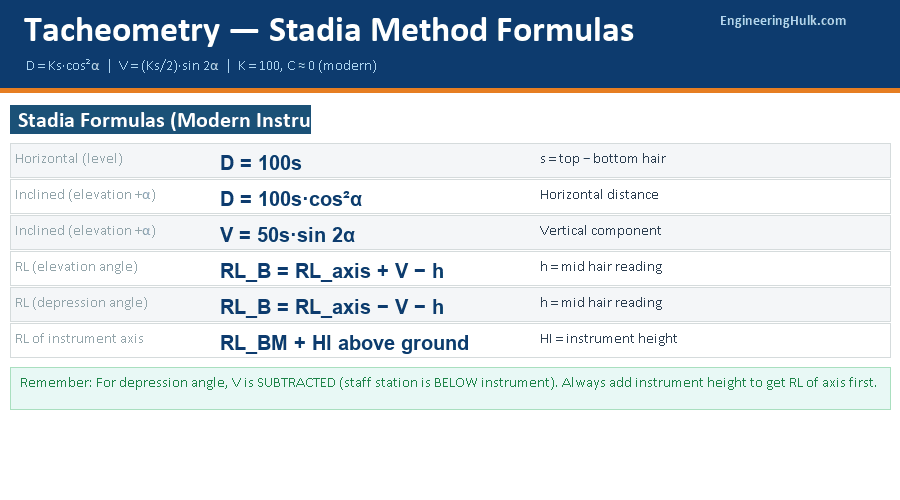
- Horizontal distance (level ground): D = Ks + C, where K = 100, s = stadia intercept, C ≈ 0 for modern telescopes.
- Inclined sights: D = Ks·cos²α; vertical component V = (Ks/2)·sin 2α.
- RL of staff station = RL of instrument axis + V − h (elevation angle); or − V − h (depression angle).
- Plane table surveying: simultaneous field observation and plotting; no booking needed.
- Four plane table methods: Radiation, Intersection, Traversing, Resection.
- Resection (three-point problem) locates an unknown station; Bessel’s method is most reliable.
1. Introduction to Tacheometry
Tacheometry (from Greek: tachos = swift, metron = measure) is a rapid method of surveying in which horizontal distances and differences in elevation are determined simultaneously by observing a graduated staff through a theodolite fitted with a stadia diaphragm. It replaces chaining in rough, hilly, or heavily wooded terrain where direct measurement is difficult.
The stadia diaphragm has three horizontal hairs: a top stadia hair, a middle hair (bisects the staff for height measurement), and a bottom stadia hair. The stadia intercept s = top reading − bottom reading. The middle reading is used to calculate the RL of the staff station.
Accuracy of tacheometry: about 1 in 1000 to 1 in 500 for horizontal distances, which is acceptable for topographic surveys, contour maps, and preliminary engineering surveys. It is not suitable for precise control work.
2. Stadia Method — Horizontal Line of Sight
Horizontal Distance & Elevation (Level Ground)
D = Ks + C
K = multiplying constant = f/i (usually 100)
s = stadia intercept = top hair reading − bottom hair reading
C = additive constant = f + d (usually 0 for internal focusing telescopes)
For modern theodolites: D = 100s
Difference in elevation = HI − middle hair reading (same as ordinary levelling)
The multiplying constant K = 100 means that 1 m of staff intercept corresponds to 100 m of horizontal distance. If stadia wires are at 1/100 m interval on the diaphragm, and the focal length is 1/100 m, then K = 100. This is fixed in the instrument and cannot be changed in the field.
3. Stadia Method — Inclined Line of Sight
Inclined Sight Formulas
Horizontal distance: D = Ks·cos²α + C·cosα
For modern instruments (C = 0): D = Ks·cos²α
Vertical component: V = (Ks/2)·sin 2α + C·sinα
For modern instruments: V = (Ks/2)·sin 2α = 50Ks·sinα·cosα
RL of staff station (elevation angle +α):
RL = RL of instrument axis + V − h
RL of staff station (depression angle −α):
RL = RL of instrument axis − V − h
Where h = middle hair reading on staff; RL of instrument axis = RL of ground station + instrument height (HI above ground)
The sign of α: elevation angle (telescope above horizontal) is positive, depression angle (telescope below horizontal) is negative. When α is positive (staff station is higher), V is added; when negative (staff station is lower), V is subtracted. The middle hair reading h is always subtracted.
4. Tangential Tacheometry
In tangential tacheometry, a plain staff without stadia marks is used. Two vertical angles α₁ and α₂ are observed to two fixed targets (usually top and bottom of a vane of height S = 2 m or 3 m on the staff).
Tangential Method Formulas
Case 1 — Both angles elevation: D = S·cosα₁·cosα₂ / sin(α₁ − α₂)
Case 2 — Both angles depression: D = S·cosα₁·cosα₂ / sin(α₁ − α₂)
Case 3 — One elevation, one depression: D = S·cosα₁·cosα₂ / sin(α₁ + α₂)
V = D·tanα₁ (to upper vane); RL from there.
Tangential tacheometry is rarely used today but was important before stadia diaphragms became standard. GATE occasionally tests the formula recognition.
5. Plane Table Surveying
Plane table surveying is a graphical method where measurements are taken and simultaneously plotted on the drawing sheet fixed to the plane table. No separate field book is needed. The key instruments are: the plane table (drawing board on a tripod), alidade (sighting rule for drawing rays), plumbing fork (centering the table over the station), and spirit level (levelling the table).
Operations: (1) Fixing — attach drawing paper to the table. (2) Centering — position the table so the plotted point is exactly over the ground station. (3) Levelling — make the table horizontal using the spirit level. (4) Orientation — make the table’s north direction consistent throughout the survey; done by backsighting a previously plotted line (back-ray method) or by magnetic compass.
Advantages: Simultaneous plotting eliminates booking errors; irregular features can be sketched in; mistakes visible immediately. Disadvantages: Cannot be used in wet or windy conditions; less precise than theodolite traverse; large areas impractical.
6. Plane Table Methods
| Method | Stations Required | Distance Measured? | Use Case |
|---|---|---|---|
| Radiation | One (detail from one station) | Yes | Open areas where all detail is visible from one point |
| Intersection | Two (inaccessible detail) | No (only baseline) | Inaccessible points (river banks, hill tops, buildings) |
| Traversing | Series of stations | Yes | Long, narrow surveys (roads, rivers, coastlines) |
| Resection | One (unknown station) | No | Locating the instrument station from known plotted points |
7. Three-Point Problem (Resection)
The three-point problem: Given three plotted control points A, B, C on the plane table, find the location of the instrument station P (not yet plotted). P is located by drawing rays from P toward A, B, and C and finding their intersection — but since P is unknown, it requires a geometric construction.
- Trial and error (Lehmann’s method): Draw rays to all three known points; they form a triangle of error. Move the estimated P according to Lehmann’s rules until the triangle reduces to a point.
- Mechanical method: Use a tracing paper to draw rays from a trial point; slide and rotate until all three rays pass through the plotted points.
- Bessel’s method (graphical): Join two of the known points with a line on the paper; draw rays to the third from each of the two known points; their intersection on the table gives the instrument station after one more ray is drawn.
Great circle method: A circle passing through any three non-collinear points is unique. The instrument station lies on the circumcircle of the triangle formed by the three known points. Drawing this circle on the plane table and locating P on it from the observed rays gives the solution.
Limitation: If P lies on the circumcircle of triangle ABC, the three rays are parallel and the problem is indeterminate — a situation called the “danger circle.” Always choose stations so P is clearly inside or outside the triangle, not on the circumcircle.
8. Worked Examples (GATE CE Level)
Example 1 — Horizontal Ground (K=100, C=0)
Staff readings from a tacheometer: top = 2.345, middle = 1.870, bottom = 1.395. Instrument height = 1.50 m, RL of instrument station = 120.500 m. Find horizontal distance and RL of staff station (horizontal sight).
Solution:
s = 2.345 − 1.395 = 0.950 m
D = 100 × 0.950 = 95.0 m
RL of instrument axis = 120.500 + 1.50 = 122.000 m
RL of staff station = 122.000 − 1.870 = 120.130 m
Example 2 — Inclined Sight (Elevation Angle) (GATE 2020 type)
From instrument station A (RL = 450.000 m, HI = 1.5 m), the following readings were taken: stadia intercept s = 1.200 m, vertical angle α = +8°30′, middle hair reading h = 2.100 m. Find horizontal distance and RL of staff station B.
Solution:
D = 100 × 1.200 × cos²(8°30′) = 120 × cos²8.5° = 120 × (0.9889)² = 120 × 0.9779 = 117.35 m
V = (100 × 1.200/2) × sin(2 × 8.5°) = 60 × sin17° = 60 × 0.2924 = 17.544 m
RL of instrument axis = 450.000 + 1.500 = 451.500 m
RL of B = 451.500 + 17.544 − 2.100 = 466.944 m
Example 3 — Depression Angle
Stadia readings: s = 0.800 m, depression angle α = 5°15′, middle hair h = 1.500 m. Instrument station RL = 300 m, HI = 1.4 m.
Solution:
D = 100 × 0.800 × cos²5.25° = 80 × (0.9958)² = 80 × 0.9916 = 79.33 m
V = (100 × 0.800/2) × sin(10.5°) = 40 × 0.1822 = 7.288 m
RL of staff station = (300 + 1.4) − 7.288 − 1.500 = 301.400 − 7.288 − 1.500 = 292.612 m
Common Mistakes
- Using the wrong sign for V in depression angle: For elevation angle, RL = axis RL + V − h. For depression, RL = axis RL − V − h. Students often add V even for depression angles.
- Forgetting cos²α in the horizontal distance formula: D = Ks·cos²α, NOT Ks·cosα. The squared cosine comes from the geometry of projection — both the intercept and the distance are projected onto the horizontal.
- Using instrument station RL instead of instrument axis RL: Always add the instrument height to the station RL before computing the staff station RL.
- Confusing stadia intercept with individual readings: s = top − bottom. The middle reading is used only for RL computation, not for distance.
- Ignoring the danger circle in resection: If the unknown station lies on the circumcircle of the three control points, the solution is indeterminate. Always check that the chosen station is safely inside or outside the triangle.
Frequently Asked Questions
What is the stadia formula in tacheometry for horizontal ground?
For horizontal line of sight: D = Ks + C. K = 100 (standard), s = stadia intercept (top − bottom hair reading), C = 0 for modern internal-focusing telescopes. So D = 100s for practical purposes.
What are the formulas for inclined sights in tacheometry?
Horizontal distance D = Ks·cos²α. Vertical component V = (Ks/2)·sin2α. RL of staff station = RL of instrument axis + V − h (elevation); or − V − h (depression). h = middle hair reading.
What are the methods of plane table surveying?
Radiation (one station, distances measured), Intersection (two stations, no distances needed), Traversing (series of stations for linear surveys), Resection (locating unknown station from three known points).
What is Bessel’s method for the three-point problem?
Bessel’s graphical method locates an unknown plane table station from three known plotted points by constructing lines through pairs of known points and finding their intersection. It is systematic and avoids the trial-and-error of Lehmann’s method.